This post is a continuation of the previous one, where I demonstrated how to perform PCA with PLINK. While PLINK’s PCA is great for quick, exploratory analysis, smartpca (part of the EIGENSOFT toolset) is more commonly used in published genetic studies.
Smartpca needs to be compiled on Linux or macOS, or alternatively installed via conda. I covered both methods in this earlier post: From EIGENSTRAT to PACKEDPED.
As before, I’ll use a small subset. The focus here is on the technical process. One key difference in this post is that I’ll perform Linkage Disequilibrium (LD) pruning, which helps reduce SNP redundancy and improves the detection of population structure in PCA.
LD Pruning
# Window size: 50 SNPs
# Step size: 5 SNPs
# LD threshold: r² > 0.2 will be pruned
plink --bfile input --indep-pairwise 50 5 0.2

# Extract the pruned SNPs into a new dataset
plink --bfile input --extract plink.prune.in --make-bed --out final
Note: If you’re working with low-coverage ancient samples, applying LD pruning directly to a mixed dataset (modern + ancient) may introduce bias, since SNP retention will favor samples with higher coverage. A better approach:
- Prune only the modern dataset.
- Use the same pruned SNP list (
plink.prune.in) to extract SNPs from the ancient dataset. - Merge both datasets.
Here’s how you can do that:
# Step 1: Prune modern samples
plink --bfile modern --indep-pairwise 50 5 0.2

# Step 2: Create pruned datasets for both groups
plink --bfile modern --extract plink.prune.in --make-bed --out pruned_modern
plink --bfile ancient --extract plink.prune.in --make-bed --out ancient_extracted

# Step 3: Merge datasets
plink --bfile pruned_modern --bmerge ancient_extracted --make-bed --out final
Converting the Dataset to EIGENSTRAT Format
Smartpca requires data in EIGENSTRAT format. Assuming your merged/pruned data is in PACKEDPED (.bed/.bim/.fam) format, you can use convertf (part of EIGENSOFT, also covered in the previous post) to convert it.
Create a parameter file named convert (or a name of your choice, adjust the parameters accordingly) with the following content:
genotypename:    final.bed
snpname:         final.bim
indivname:       final.fam
outputformat:    EIGENSTRAT
genotypeoutname: pca.geno
snpoutname:      pca.snp
indivoutname:    pca.ind
Now run:
convertf -p convert
This will generate the three required input files for smartpca: pca.geno, pca.snp, and pca.ind.
Creating the Smartpca Parameter File
Like most Reich Lab tools, smartpca uses a parameter file to specify input and output options. Here’s a minimal example:
genotypename:     pca.geno
snpname:          pca.snp
indivname:        pca.ind
evecoutname:      pca.evec
evaloutname:      pca.eval

altnormstyle:     NO
numoutevec:       10
numoutliter:      0
lsqproject:       YES
numthreads:       5
lsqproject: YES enables projection mode, meaning projected samples don’t influence the PCA axes. In this example, all samples are high-coverage modern individuals, so projection isn’t technically needed, but I demonstrate it here for completeness. Save the parameter file with a name like pca_param (no extension).
To project samples, you’ll need to modify the .ind file of your EIGENSTRAT dataset. Change the third column from Case to P:
      ...
      2032:TLA018.HO M       Case
      2033:TLA019.HO M       P
      2034:TLA020.HO M       Case
      ...
Running Smartpca
Now we run smartpca with:
smartpca -p pca_param
This generates two files: pca.eigenval (lists how much variance each eigenvector explains) and pca.evec (contains sample IDs and principal component values).
Preparing for Plotting
To make the output compatible with the attached script from the below, convert the .evec file to CSV:
awk 'NR>1 { $NF=""; sub(/[ \t]+$/, ""); gsub(/[ \t]+/, ","); print }' pca.evec > smartpca.csv
At this point, you have two options:
- Use the Python plotting script from my previous PLINK PCA tutorial
- Use Vahaduo for a browser-based, interactive visualization (explained below)
Option 1: Plotting with Python
If you’ve already set up Python and created the plotting script from the PLINK tutorial, you can use it directly. You’ll need to:
- Create a labels file from your
.indfile:
awk 'NR==FNR {map[$1]=$3; next} {print map[$2]}' pca.ind final.fam > labels
- Run the plotting script with
smartpca.csvandlabels:
This is the resulting plot for an European subset:
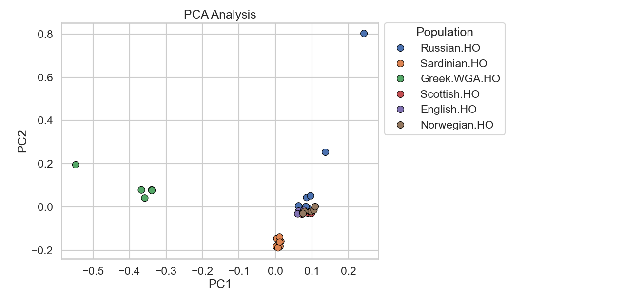
Note: The apparent spread of some samples (e.g., the Russian outlier on PC2) is a plotting artifact from using a small subset. With larger reference panels (1000+ samples), PCA axes become more stable and outliers appear less extreme. This is why published aDNA studies project ancient samples onto axes defined by large modern reference sets.
Option 2: Plotting with Vahaduo (No Coding Required)
Vahaduo is a web-based tool that can generate interactive 2D and 3D PCA plots without any programming. However, it requires population labels to be embedded directly in the CSV file.
Preparing the file for Vahaduo:
Your current smartpca.csv file looks like this:
...
11788:HGDP00553.HO,0.0136,0.0104,0.0353,-0.0510,...
11789:HGDP00554.HO,0.0136,0.0107,0.0334,-0.0494,...
11790:HGDP00555.HO,0.0137,0.0104,0.0346,-0.0511,...
...
Vahaduo groups samples by the text before the : character. We need to replace the numerical FIDs with population labels. Here’s an awk command that does this automatically (adjust filenames if needed):
# When I refer to an .ind file, I always mean the original version from the dataset as it was downloaded (aside from the prefix used here)

awk -F',' -v OFS=',' '
  NR == FNR {
    line = $0
    gsub(/^[[:space:]]+/, "", line)
    if (line == "") next

    split(line, a, /[[:space:]]+/)
    if (a[1] == "" || a[3] == "") next

    label = a[3]
    sub(/\.(AG|DG|HO|SG)$/, "", label)
    pop[a[1]] = label
    next
  }

  {
    if (split($1, parts, ":") >= 2 && (parts[2] in pop))
      $1 = pop[parts[2]] ":" parts[2]
    print
  }
' data.ind smartpca.csv > smartpca_with_labels.csv
This transforms the file to (for example):
...
Papuan:HGDP00553.HO,0.0136,0.0104,0.0353,-0.0510,...
Papuan:HGDP00554.HO,0.0136,0.0107,0.0334,-0.0494,...
Papuan:HGDP00555.HO,0.0137,0.0104,0.0346,-0.0511,...
...
Using Vahaduo:
- Go to https://vahaduo.github.io/custompca/
- Navigate to the PCA tool
- Paste the contents of
smartpca_with_labels.csvinto the “PCA Data” section - Click “Plot PCA” in the “PCA plot” section to generate the visualization
Advantages of Vahaduo Plotting:
- No Python set-up required
- Interactive plots (zoom, pan, rotate in 3D)
- Hover over points to see sample details
- Quick exploratory analysis
- Saving plots
Vahaduo can also run a distance-minimizing heuristic to fit a target sample as a mix of chosen source groups, and the CSV produced here works with that feature. The main issue is that PCA compresses many SNPs into a relatively small set of principal components, so the model operates on a simplified and linear view of the underlying data. More fundamentally, PCA-based modeling conflates proximity in a reduced linear space with ancestry. The tool simply finds mixture proportions that minimize Euclidean distance in PCA space, it is heuristic curve-fitting at best, not ancestry inference, and I don’t consider PCA-based models to be proof of anything. The reality revealed by formal statistics like F4-admixture tests is often extremely different, as these methods explicitly test for shared genetic drift patterns that indicate true phylogenetic relationships rather than mere spatial proximity in a dimension-reduced projection.