Running f4-Statistics with ADMIXTOOLS2 in R

This post covers how to run f4-statistics using the admixtools package for R. Compared with the original ADMIXTOOLS workflow, the R implementation is more convenient for testing multiple population combinations because it can be used interactively, without repeatedly editing parameter files. It is also much faster in practice, which makes it possible to work directly with the full AADR dataset without creating subsets.

What are f4-statistics?

F4-statistics measure asymmetry in allele sharing among four populations. For four populations $A$, $B$, $C$, and $D$, the statistic is written as:

Here, $a_i$, $b_i$, $c_i$, and $d_i$ are the allele frequencies of populations $A$, $B$, $C$, and $D$ at SNP $i$, and $n$ is the number of SNPs used in the calculation.

Mathematically, the statistic is an average product of allele-frequency differences. In population-genetic terms, it tests whether allele sharing is symmetric across the quartet: does one population share the same amount of drift with two comparison populations, or is there a detectable excess affinity on one side? Under a simple tree model with no admixture connecting the two sides of the comparison, the statistic is expected to be zero. A significantly positive or negative value indicates asymmetric allele sharing, usually implying that the four populations do not fit that simple tree.

This might sound more complicated than it is. In essence you’re testing whether populations form a simple tree or show deviations consistent with gene flow between populations.

Interpreting f4-statistics (with A as deep outgroup)

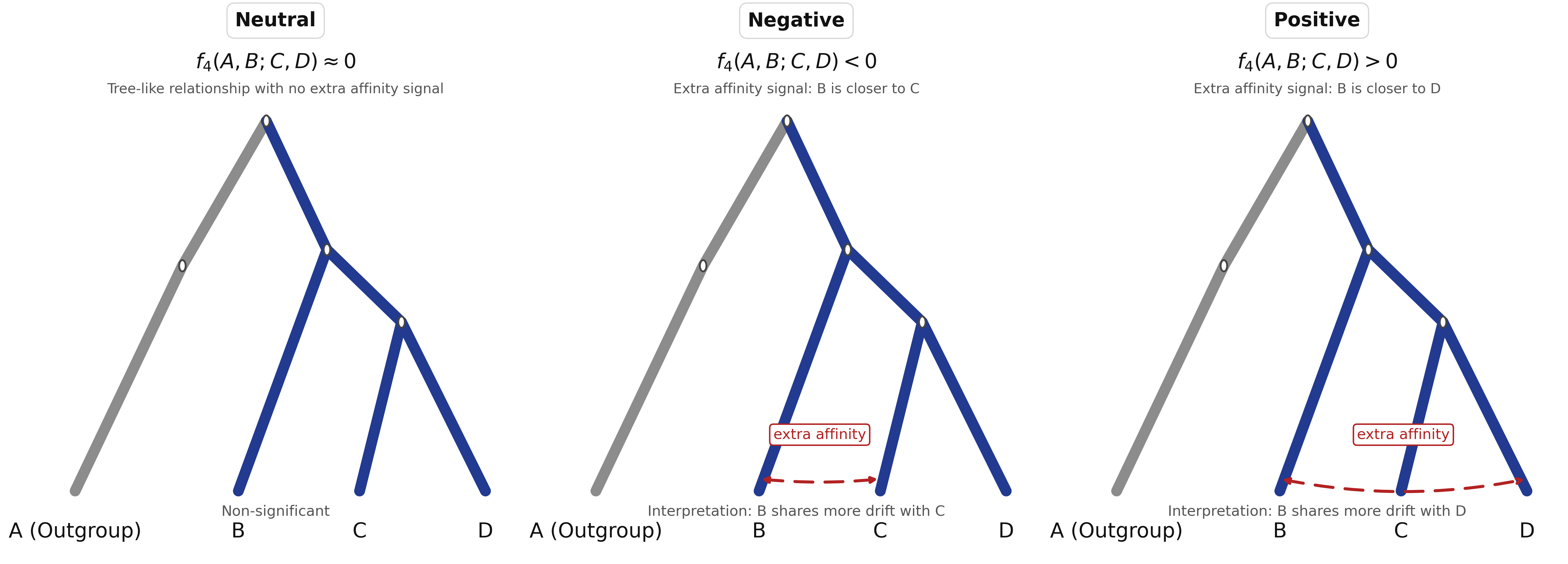
When using a deep outgroup in position $A$, such as Mbuti, the sign tells you which populations share more drift:

• Positive $f_4(A,B;C,D)$: population $B$ shares more drift with $D$ than with $C$
• Negative $f_4(A,B;C,D)$: population $B$ shares more drift with $C$ than with $D$
• Zero or non-significant: $B$ shares similar amounts of drift with $C$ and $D$, consistent with a simple tree

Because f4-statistics are ordered, changing the population order can change the sign. Swapping the two populations in the first pair, or swapping the two populations in the second pair, reverses the sign:

This does not change the underlying relationship being tested, but it changes whether the result is reported as positive or negative. In particular, swapping $A$ and $B$ reverses the sign and changes which population is being interpreted as sharing more drift with $C$ or $D$.

If you are new to f4-statistics, the easiest convention is to place a deep outgroup, such as Mbuti, in position $A$, keep the population you want to interpret in position $B$, which corresponds to pop2 in admixtools2, and then compare whether it shares more drift with $C$ or $D$.

Statistical significance is assessed using z-scores. The conventional threshold is $|z| > 3$, though $|z| > 2$ can also be useful for exploratory analysis.

Setting Up R and Admixtools

First, install R and the required dependencies. For Ubuntu/Debian:

sudo apt update -y

sudo apt install -y r-base r-base-dev build-essential \
  libcurl4-openssl-dev libssl-dev libxml2-dev libgsl-dev

Next, start R by running R in your terminal, then install admixtools:

install.packages("remotes")
remotes::install_github("uqrmaie1/admixtools")

Running f4-statistics

I’ll use the AADR dataset, the most comprehensive curated collection of ancient and modern genomic samples. Since Admixtools works with EIGENSTRAT files and AADR is distributed in this format, the dataset can be used directly without preprocessing. For download instructions, see: Download Ancient & Modern DNA (AADR Tutorial).

If you want to also analyze your own DNA (23andMe, AncestryDNA, FamilyTreeDNA, MyHeritage, Living DNA) alongside AADR, see the Raw DNA to AADR toolkit, which handles the conversion and merge end-to-end.

Then, navigate to the directory containing your downloaded AADR dataset files (.geno, .snp, .ind) and start R:

 # move into the folder so the files can be loaded without specifying paths
cd /path/to/aadr/dataset
R

Load the previously installed admixtools library and dataset:

library(admixtools)

# Specify the file prefix (without extensions)
# If your files are named v62.0_HO_public.geno/.snp/.ind
# use only the prefix:
data = "v62.0_HO_public"

When specifying populations in f4-statistics, use the exact population labels from the third column of your .ind file, the function will automatically include all samples assigned to that population label.

Now we can run f4-statistics. You’ll need specific hypotheses about population relationships to test. I’ll demonstrate three examples that illustrate different outcomes.

In the examples below, pop1 through pop4 correspond to populations A, B, C, and D respectively, where (A, B) and (C, D) form the two pairs being compared.

Example 1: Do Yamnaya Share More Drift with EHG than WHG?

For this test, we’ll use Mbuti as the outgroup (position A), Yamnaya in position $B$, a WHG-related sample (Italian Epigravettian) in position $C$, and an EHG-related sample (Latvia Mesolithic) in position $D$.

Run the following in your R session:

f4(data, pop1="Mbuti.HO", pop2="Russia_Samara_EBA_Yamnaya.AG", pop3="Italy_Epigravettian_alt.AG.BY.AA", pop4="Latvia_Mesolithic_oEHG.AG")

The result shows:

  pop1     pop2                  pop3  pop4      est      se     z       p     n
  <chr>    <chr>                 <chr> <chr>   <dbl>   <dbl> <dbl>   <dbl> <dbl>
1 Mbuti.HO Russia_Samara_EBA_Ya… Ital… Latv… 0.00245 9.17e-4  2.67 0.00751 49477

The z-score of 2.67 falls just below the conventional significance threshold of 3, but the result is still informative. While some use a stricter threshold of |z| > 3, others consider |z| > 2 sufficient for exploratory analysis, particularly when the direction of the effect is theoretically motivated. The positive value indicates that Yamnaya shares more drift with EHG than with the WHG sample from Villabruna. The output also reports n, which is the number of SNPs used in the calculation. Here, roughly 49k SNPs contributed to the statistic. In general, larger SNP counts increase accuracy, making it easier to reach |z| > 3.

Re-running a closely related version of the Yamnaya test on a denser dataset, and using Russia_Samara_EN_Mesolithic in place of the previous EHG-related population, gives a strongly significant result (est = 0.00210, z = 10.4, p = 2.87e-25, n = 843572). With Mbuti as a deep outgroup, the positive sign again indicates that Yamnaya shares more alleles with Russia_Samara_EN_Mesolithic (position $D$) than with Italy_NordEst_Epigravettian (position $C$). So this is not just suggestive anymore: it is strong evidence of asymmetric allele sharing in this quartet.

Example 2: Do Anatolian Neolithic Farmers Share More Drift with Sardinians or French?

f4(data, pop1="Mbuti.HO", pop2="Turkey_Marmara_Barcin_N.AG", pop3="Sardinian.HO", pop4="French.HO")

The result shows:

  pop1     pop2               pop3  pop4       est      se     z        p      n
  <chr>    <chr>              <chr> <chr>    <dbl>   <dbl> <dbl>    <dbl>  <dbl>
1 Mbuti.HO Turkey_Marmara_Ba… Sard… Fren… -0.00233 1.25e-4 -18.6 2.49e-77 155527

This result is highly significant with a z-score of -18.6. The negative value indicates that Anatolian Neolithic farmers (population $B$) share significantly more drift with Sardinians (population $C$) than with the French (population $D$). This is consistent with Sardinians retaining the highest proportion of Neolithic farmer ancestry in Europe.

If we replaced Sardinians with Han Chinese, the test would again be highly significant, showing strong drift sharing between Barcin Neolithic and French, but the signal would imply something else. Instead of detecting differences in Neolithic farmer ancestry within Europe, it would mainly reflect the much deeper contrast between Western Eurasian and East Asian ancestry: Anatolian Neolithic farmers and French share far more ancestry with each other than either does with Han Chinese.

The f4-statistic itself only reports allele-sharing asymmetry in the quartet. It does not recover “Neolithic farmer ancestry” as a separate component on its own. The historical interpretation comes from the population choice: here, Sardinians and French both share a farmer-related baseline, and the statistic detects Sardinian excess affinity to Anatolian Neolithic farmers relative to French.

Example 3: Comparing French, Scottish, and Norwegian Relationships

f4(data, pop1="Mbuti.HO", pop2="French.HO", pop3="Scottish.HO", pop4="Norwegian.HO")

The result shows:

  pop1     pop2      pop3        pop4             est      se     z     p      n
  <chr>    <chr>     <chr>       <chr>          <dbl>   <dbl> <dbl> <dbl>  <dbl>
1 Mbuti.DG French.HO Scottish.HO Norwegian.HO 1.92e-4 2.05e-4 0.941 0.347 155583

The f4-statistic is non-significant (z = 0.941), meaning this particular ordered test does not detect excess affinity of French to either Scottish or Norwegian. With Mbuti as the outgroup and French in position B, the test only asks whether French share more drift with Scottish or with Norwegian, it does not address whether Scottish and Norwegian themselves share excess affinity with each other. As we’ll see when rotating the populations below, a non-significant result in one orientation does not rule out asymmetries that become visible in another.

To explore the relationship more completely, you can rotate which population is placed in position $B$. This changes the question being asked: instead of only asking whether French are closer to Scottish or Norwegian, you can also ask whether Scottish are closer to French or Norwegian, and whether Norwegian are closer to French or Scottish.

For example:

# Are French closer to Scottish or Norwegian?
f4(data, pop1="Mbuti", pop2="French", pop3="Scottish", pop4="Norwegian")

# Are Scottish closer to French or Norwegian?
f4(data, pop1="Mbuti", pop2="Scottish", pop3="Norwegian", pop4="French")

# Are Norwegian closer to Scottish or French?
f4(data, pop1="Mbuti", pop2="Norwegian", pop3="Scottish", pop4="French")

Note: These rotated examples use AADR v66 labels, which no longer include the .HO suffix. The interpretation is unchanged.

When running the f4-statistic with Norwegian in position $B$:

  pop1  pop2      pop3     pop4         est       se     z          p      n
  <chr> <chr>     <chr>    <chr>      <dbl>    <dbl> <dbl>      <dbl>  <dbl>
1 Mbuti Norwegian Scottish French -0.000861 0.000195 -4.42 0.00000980 678870

The negative sign, with $A$ as a deep outgroup, indicates that Norwegian shares significantly (|z| = 4.42) more drift (est = -0.000861) with Scottish than with French. This demonstrates why the population in position $B$ matters: the earlier French-centered test asked whether French are closer to Scottish or Norwegian, while this test asks whether Norwegian is closer to Scottish or French. These are related questions, but they are not the same ordered comparison.

When running the f4-statistic with Scottish in position $B$:

  pop1  pop2     pop3      pop4         est       se     z      p      n
  <chr> <chr>    <chr>     <chr>      <dbl>    <dbl> <dbl>  <dbl>  <dbl>
1 Mbuti Scottish Norwegian French -0.000602 0.000258 -2.34 0.0195 678870

The negative sign points in the same direction: Scottish tendentially share more drift with Norwegian than with French. However, the result is below the stricter $|z| > 3$ threshold (|z| = 2.34). In context, it is still consistent with the broader expectation that Scottish and Norwegian are more closely related to each other than either is to French.

Conclusion

F4-statistics are excellent for detecting admixture signals and differential relatedness, but they should not be overinterpreted. A significant f4-statistic tells you that four populations do not fit a simple tree and that one pair shows excess allele sharing relative to the other, but it does not tell you the direction of gene flow, whether the connection is direct or indirect, or the ancestry proportions involved. For that kind of admixture modeling, qpAdm is the next step.

At the same time, f4-statistics are also useful for asking whether populations can be placed on a simple tree in a way that is consistent with the data. When an f4-statistic is significantly different from zero, that proposed tree-like relationship is rejected. For this reason, f4-statistics are also needed for qpGraph.